The maser goes mainstream: Diamond microwave lasers

Posted on Fri 23 March 2018 in masers, quantum • Tagged with masers, quantum, diamond

My colleague Juna and myself had a great time filming with the Nature Video guys Elizabeth Gibney, Noah Baker and Lizzy Brown. My kids loved 'Disco Einstein' at the end of the video.


The maser goes mainstream: Diamond microwave lasers

Posted on Wed 21 March 2018 in masers • Tagged with masers, quantum, diamond

Our paper 'Continuous-wave room-temperature diamond maser' was published in Nature and also made the cover.


IBM Ups Pressure on Rivals With Quantum Computer Prototype

Posted on Fri 10 November 2017 in quantum • Tagged with quantum

In the news again ... I was interviewed by Jeremy Kahn of Bloomberg for an article on IBM's announcement of 50-qubit quantum computer:

IBM Ups Pressure on Rivals With Quantum Computer Prototype


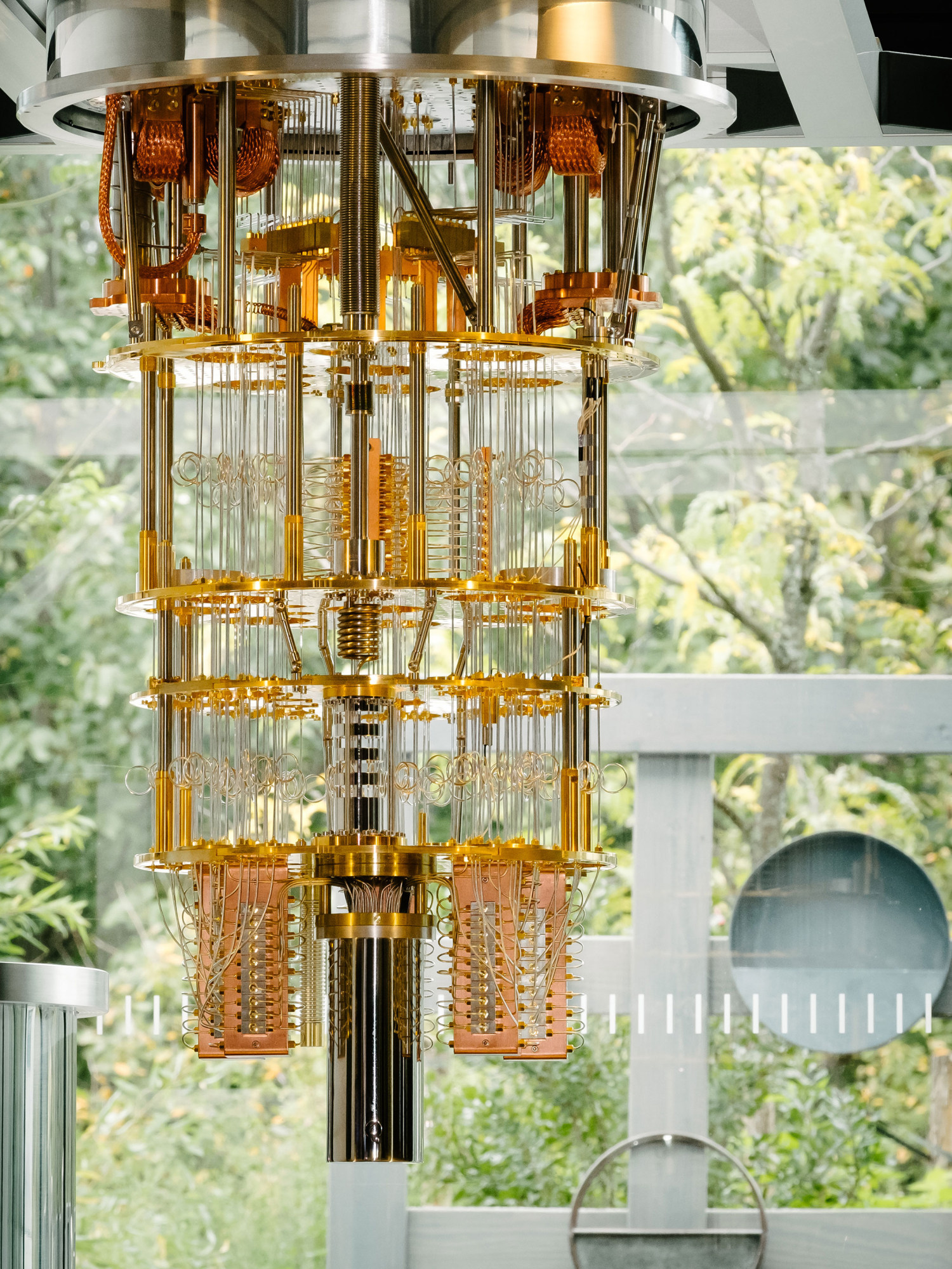
An IBM cryostat refrigeration system for a quantum system.
Photographer: Graham Carlow/IBM


Quantum computing breakthrough: Imperial scientist (me) reveals latest findings

Posted on Wed 25 October 2017 in quantum • Tagged with masers, quantum

In the local news ...

Quantum computing breakthrough: Imperial scientist (me) reveals latest findings
(article by Colin Smith)


Room-Temperature Cavity Quantum Electrodynamics

Posted on Sat 30 September 2017 in quantum • Tagged with masers, quantum

My new paper in npj Quantum Information on cavity quantum electrodynamics using masers is available free (open access) here:

Room-temperature cavity quantum electrodynamics with strongly coupled Dicke states

In this work, we managed to achieve strong-coupling at room-temperature with a photo-excited spin-ensemble. Similar studies have been presented previously with ensembles of paramagnetic ions, but this is the first time an almost pure collective quantum state had been initialised. Of the \(10^{\sf 15}\) pentacene molecules, over 90% were prepared in the excited state.

This was a fun paper. Realising we were operating in the strong-coupling regime of cavity quantum electrodynamics, for me, was a milestone.


Science Museum Lates (Space)

Posted on Thu 10 August 2017 in masers • Tagged with masers, space

On the evening of August 30th (18:45–22:00), we will be presenting our 'Amazing Masers' exhibit at the space themed Science Museum 'Lates' event, where the Royal Society, BBC, Wellcome Trust and the Open University team up with the Science Museum to bring you the best in UK space research. Strictly over 18s only!

Find out more here.

Image credit: European Space Agency & NASA


MEEP modelling: Square Cavity – Part 2

Posted on Tue 25 July 2017 in MEEP • Tagged with meep, electromagnetic

If we inspect the output from meep that we saved in file square.ctl:

-----------
Initializing structure...
Working in 2D dimensions.
Computational cell is 1 x 1 x 0 with resolution 21
     block, center = (0,0,0)
          size (1,1,1e-20)
          axes (1,0,0), (0,1,0), (0,0,1)
          dielectric constant epsilon diagonal = (1,1,1)
time for set_epsilon = 0.00246215 s
-----------
Meep progress: 1265.7857142857142/2005.0 = 63.1% done in 4.0s, 2.3s to go
on time step 53163 (time=1265.79), 7.52429e-05 s/step
harminv0:, frequency, imag. freq., Q, |amp|, amplitude, error
harminv0:, 0.49965027602074025, 6.962901950688442e-8, -3587945.6551254354, 0.07777794402701167, 0.0024368236485488148+0.07773976117518522i, 2.1971119199697203e-8+0.0i
harminv0:, 0.7067768851898223, -7.597594046763396e-8, 4651320.410379862, 0.03547170560103376, -0.00560172786233135-0.03502659765382288i, 1.6310167415083462e-8+0.0i
harminv0:, 0.997198615390459, -2.2874161068410783e-8, 21797490.46113849, 0.30571523921562116, 0.30557359296981657-0.009305201135996685i, 4.379556711147102e-9+0.0i
harminv0:, 1.1157886868016782, -7.198145589973213e-9, 77505287.4976533, 0.18504732775678, -0.06019929248036505-0.17498159530301646i, 2.0145105671454234e-9+0.0i
harminv0:, 1.4115657086248123, 9.691822540596569e-8, -7282251.107632874, 0.09323703957434044, 0.08941825563599501-0.02641062489989536i, 1.2346770754915476e-8+0.0i
harminv0:, 1.490528739827691, 1.4909785346550363e-7, -4998491.611995442, 0.04358290725731711, 0.001576775048424593-0.043554375043691876i, 2.8521991089171737e-8+0.0i
harminv0:, 1.572707606509909, -8.635811826769853e-8, 9105731.100084461, 0.03510133186423594, -0.03341229909079056-0.01075740526850139i, 1.1398999164323018e-8+0.0i
harminv0:, 1.7956590548227003, 2.713483475275414e-7, -3308770.941824962, 0.0173063963599404, 0.017267776387618082-0.0011555317367245932i, 3.265935897573454e-8+0.0i
harminv0:, 1.9774955614133072, -3.2803139027426844e-7, 3014186.4773366884, 0.01085226263124576, -0.010634565235754036-0.002162782112008712i, 9.627394698484882e-8+0.0i
run 0 finished at t = 2005.0 (84210 timesteps)

Elapsed run time = 12.9194 s

we see that some resonant frequencies have been generated (look for lines beginning with harminv0) Let's extract the frequencies with the unix command grep harminv0 square.out | sed 's/,//g' | gawk '{printf "%.4f\n", $2}', which looks for lines containing the text harminv, removes commas and then takes the second column and prints the value to 4 decimal places:

0.4997
0.7068
0.9972
1.1158
1.4116
1.4905
1.5727
1.7957
1.9775

We ignore the first entry 0.000 since it is the result of printing the second column of the legend harminv0:, frequency, imag. freq., Q, |amp|, amplitude, error. Due to the simple geometry we can also calculate the frequency of the modes analytically using the expression

$$ f = \tfrac{1}{2} \sqrt{n_x^2 + n_y^2} $$

where \(n_x\) and \(n_y\) are the number of half-waves in the \(x\) and \(y\) directions. This can be derived from the wavenumber \(k^2 = k_x^2 + k_y^2 = \pi^2(n_x^2+n_y^2)\) and \(f = \omega/2\pi = ck/2\pi\). Since \(c=1\) in meep, then

$$ f = \frac{ck}{2\pi} = \frac{\pi\sqrt{n_x^2+n_y^2}}{2\pi} = \tfrac{1}{2} \sqrt{n_x^2 + n_y^2} $$
meep \(n_x\) \(n_y\) \(f\) \(f\) \(\Delta f\)
0.4996 0 1 \(\tfrac{1}{2}\sqrt{0^2 + 1^2} = \tfrac{1}{2}\) 0.500 0.0004
0.7068 1 1 \(\tfrac{1}{2}\sqrt{1^2 + 1^2} = \tfrac{\sqrt{2}}{2}\) 0.707 0.0002
0.9972 0 2 \(\tfrac{1}{2}\sqrt{0^2 + 2^2} = 1\) 1.000 0.0028
1.1158 1 2 \(\tfrac{1}{2}\sqrt{1^2 + 2^2} = \tfrac{\sqrt{5}}{2}\) 1.118 0.0022
1.4116 2 2 \(\tfrac{1}{2}\sqrt{2^2 + 2^2} = \sqrt{2}\) 1.414 0.0024
1.4905 0 3 \(\tfrac{1}{2}\sqrt{0^2 + 3^2} = \tfrac{3}{2}\) 1.500 0.0095
1.5727 1 3 \(\tfrac{1}{2}\sqrt{1^2 + 3^2} = \tfrac{\sqrt{10}}{2}\) 1.581 0.0083
1.7957 2 3 \(\tfrac{1}{2}\sqrt{2^2 + 3^2} = \tfrac{\sqrt{13}}{2}\) 1.803 0.0073
1.9775 0 4 \(\tfrac{1}{2}\sqrt{0^2 + 4^2} = 2\) 2.000 0.0225

If we set the excitation to \(E_z\) then we do not excite as many modes. This is because the boundary conditions do not permit either \(n_x = 0\) or \(n_y\) = 0.

meep \(n_x\) \(n_y\) \(f\) \(f\) \(\Delta f\)
0.7068 1 1 \(\tfrac{1}{2}\sqrt{1^2 + 1^2} = \tfrac{\sqrt{2}}{2}\) 0.707 0.0002
1.1158 1,2 2,1 \(\tfrac{1}{2}\sqrt{1^2 + 2^2} = \tfrac{\sqrt{5}}{2}\) 1.118 0.0022
1.4116 2 2 \(\tfrac{1}{2}\sqrt{2^2 + 2^2} = \sqrt{2}\) 1.414 0.0024
1.5727 1,3 3,1 \(\tfrac{1}{2}\sqrt{1^2 + 3^2} = \tfrac{\sqrt{10}}{2}\) 1.581 0.0083
1.7957 2,3 3,2 \(\tfrac{1}{2}\sqrt{2^2 + 3^2} = \tfrac{\sqrt{13}}{2}\) 1.803 0.0073

MEEP modelling: Square Cavity – Part 1

Posted on Thu 20 July 2017 in MEEP • Tagged with meep, electromagnetic

Assuming that you have already installed MEEP, attempted some of the examples and followed the tutorials, let's try a simple problem of finding the frequencies and fields of the eigenmodes of a two-dimensional square of air/vacuum surrounded by perfect electric conductor (PEC) boundaries.

MEEP can use the Scheme programming language (a dialect of Lisp) as an interface to the nuts & bolts of the code. You essentially code the problem you want to solve by writing a program.

So let's get started. Open a new file called square.ctl in your favourite text editor then copy & paste the following snippets of code.

; Eigenmodes of a 2D square cavity

Anything after a colon is a remark. Always handy to remind yourself what the code does:

The first thing we need to do is define the geometry-lattice which defines the extent and dimensionality of our computational space. Here, we define a two-dimensional square with sides of length 1 in meep units (more on those later) in the \(x\)-\(y\) plane and with zero thickness i.e. no-size in the \(z\)-direction:

(set! geometry-lattice (make lattice (size 1 1 no-size)))

The next step – and sometimes the trickiest – is to define the geometry, the position, shape, size and material of structures within the computational space. For this simple case we just define a zero-thickness square of air/vacuum with the same dimensions:

(set! geometry (list
        (make block (center 0 0 0) (size 1 1 no-size) (material air))
))

Set the resolution, the number of cells per unit distance (a conservative value to keep simulation time low):

(set-param! resolution 20)

Define some parameters for the centre frequency and bandwidth of the point-source gaussian pulse using define-param:

(define-param fcen 1) ; pulse center frequency                            
(define-param df 2)  ; pulse width (in frequency)

Define the source; in this case a gaussian pulse with centre frequency fcen = 1.5 and bandwidth fwidth = 3.0, positioned at \(x\)=0.25, \(y\)=0.25 and exciting the \(E_x\) component of the electric field:

(set! sources (list
               (make source
                 (src (make gaussian-src (frequency fcen) (fwidth df)))
                 (component Ex) (center 0.33 0.33) )));

Run the FDTD simulation for the duration of the source pulse (exercise: work it out), then continue for a sufficient length of time. The following statement run-sources does just that. At the beginning it saves a permittivity file (which isn't much help for us at the moment), then after the source pulse, the after-sources command runs harminv which analyses the \(E_x\) time-domain data collected at point \(x\)=0.25, \(y\)=0.25 using harmonic inversion to estimate the resonant frequencies (and Q-factors) of any resonances. The command then runs the FDTD simulation for an additional 200 meep time units, which happen to be 200 periods of the pulse centre frequency fcen (more on those later).

(run-sources+ 200
    (after-sources (harminv Ex (vector3 0.033 0.033) fcen df)))

Once you've copy & pasted all of these sections into your text editor, save it as square.ctl or download it from here. Then get MEEP to process it using the command-line, something like meep square.ctl | tee square.out. The pipe (tee) echoes the output into a file.

You should (all being well) see some output text, showing that meep has executed the instructions in square.ctl and finished without errors. Something like:

-----------
Initializing structure...
Working in 2D dimensions.
Computational cell is 1 x 1 x 0 with resolution 21
     block, center = (0,0,0)
          size (1,1,1e-20)
          axes (1,0,0), (0,1,0), (0,0,1)
          dielectric constant epsilon diagonal = (1,1,1)
time for set_epsilon = 0.00232601 s
-----------
Meep progress: 1308.7380952380952/2003.3333332538605 = 65.3% done in 4.0s, 2.1s to go
on time step 54967 (time=1308.74), 7.27747e-05 s/step
harminv0:, frequency, imag. freq., Q, |amp|, amplitude, error
harminv0:, 0.49964982320796947, -6.387829272631824e-7, 391095.1607212498, 0.013285597622112183, -0.007052720387953484-0.011259051438998675i, 2.3287614080376595e-7+0.0i
harminv0:, 0.7067779190836112, 1.691710912831851e-6, -208894.41385126952, 0.005994921731086088, -0.002373006416742774+0.0055052635820590674i, 5.339765273626355e-7+0.0i
harminv0:, 0.9971987526065739, 1.6536690637644267e-7, -3015109.7775770864, 0.07795287534323195, 0.03595210583102817-0.06916716605870166i, 4.795095158586878e-8+0.0i
harminv0:, 1.1157887584886936, -1.399235272127685e-7, 3987137.7627295624, 0.06361903731428901, -0.044370834218134786-0.04559178631709551i, 3.2413084735784084e-8+0.0i
harminv0:, 1.4115657480682742, 4.0255510363580226e-8, -17532577.966584906, 0.0940011704004871, 0.06407402923620237+0.06878036648709931i, 1.0281322317081819e-8+0.0i
harminv0:, 1.4905289327310962, 9.500093703078488e-8, -7844811.742478356, 0.06351546181488635, 0.06351074111746435-7.743721771272548e-4i, 1.520738285961082e-8+0.0i
harminv0:, 1.5727074536238252, 2.96402781900332e-9, -265299037.26623282, 0.07776848493442345, 0.04957534656074576-0.059918463451407035i, 1.3776718980993644e-8+0.0i
harminv0:, 1.7956591793170913, -3.5930574726457174e-8, 24987899.483762957, 0.14467020137786865, -0.14410062932432377+0.012824811696352946i, 5.64638078279913e-9+0.0i
harminv0:, 1.9774963650323654, 5.985926891666783e-10, -1651787935.9546697, 0.32586317906949197, 0.13754120415113452+0.2954136568168976i, 2.5490377382288595e-9+0.0i
run 0 finished at t = 2003.3333333333333 (84140 timesteps)

Elapsed run time = 12.8566 s

So, what actually happened here? MEEP did a few things: setting up arrays representing the materials and boundary conditions of the problem, running the problem for an additional time of 200 after the sources and then listing the resonant frequencies detected by a probe monitoring the \(x\)-component of the electric field at position \((0.05, 0.05)\).

We have some data to analyze, onto the next post ...

Introduction to MEEP

Posted on Thu 20 July 2017 in MEEP • Tagged with meep, electromagnetic

MEEP is a free (GNU GPL) finite-difference time-domain package developed by MIT for modelling electromagnetic systems.

It has some useful features such as:

  • 1D, 2D, 3D and cylindrical coordinates
  • Parallelism using the MPI standard
  • Arbitrary anisotropic electric permittivity ε and magnetic permeability μ
  • Dispersive ε(ω) and μ(ω) (including loss/gain) and nonlinear (Kerr & Pockels) dielectric and magnetic materials, and electric/magnetic conductivities σ.
  • PML absorbing boundaries and/or perfect conductor and/or Bloch-periodic boundary conditions.
  • Exploitation of symmetries to reduce the computation size — even/odd mirror symmetries and 90°/180° rotations.
  • Scriptability — either via a Scheme scripting front-end (as in libctl and MPB), or callable as a C++ library; a Python interface is also available.
  • Field output in the HDF5 standard scientific data format, supported by many visualization tools.
  • Arbitrary material and source distributions.
  • Field analysis including flux spectra, Maxwell stress tensor, frequency extraction, local density of states and energy integrals, near to far field transformations – all completely programmable.
  • Multi-parameter optimization, root-finding, integration, etcetera (via libctl).

I've been using MEEP for quite a few years and recently realised I had a whole bunch of different systems I had been modelling that would probably never see the light of day, but might be useful to others.

So I shall slowly be adding these MEEP examples to the blog. In the meantime, I recommend checking out MEEP – install it and go through the tutorials.


Royal Society Summer Exhibition 2017

Posted on Wed 19 July 2017 in masers • Tagged with masers, royal society

We (a joint venture between Imperial College London and University College London) recently exhibited at the Royal Society Summer Exhibition 2017.

Our exhibit 'Amazing Masers' exhibit showcased our room-temperature maser, the first time it has been outside a lab. We also encouraged visitors to build pentacene, p-terphenyl and other molecules and test drive a robotic mars rover on a CNC machined model of the surface of Mars via a video feed.

Here's our video that explains what masers are, what they do and what they could do:

Thanks to our volunteers we had a very successful week with only a few minor technical hitches. We hope that our visitors enjoyed the exhibit and learnt about masers and their new exciting future.